1 Introduction
GitHub地址
文章链接
大佬Evan E. Eichler团队基于Miropeats开发的用于基因组结构变异可视化的工具SVbyEye,使用ggplot2绘图语法实现。

2 PAF格式输入文件
需要输入的文件是PAF格式的,官方使用的比对软件是minimap2 (version >=2.24),但是任何sequence-to-sequence比对生成的结果只要可以转换为PAF格式都可以。如果使用minimap2进行比对的话不能设置-a这个参数,这个参数生成的结果是SAM格式;但是要设置-c这个参数将 CIGAR strings导出为PAF文件中的cg标签;建议设置–eqx参数将CIGAR string标记为=/X,这个是用来表示match/mismatch的。
2.1 assembly-to-reference
1
| minimap2 -x asm20 -c –eqx –secondary=no {reference.fasta} {query.fasta} > {output.alignment}
|
2.2 sequence-to-sequence
1
| minimap2 -x asm20 -c –eqx –secondary=no {target.fasta} {query.fasta} > {output.alignment}
|
2.3 all-versus-all
1
| minimap2 -x asm20 -c –eqx -D -P –dual=no {input.multi.fasta} {input.multi.fasta} > {output.ava.alignment}
|
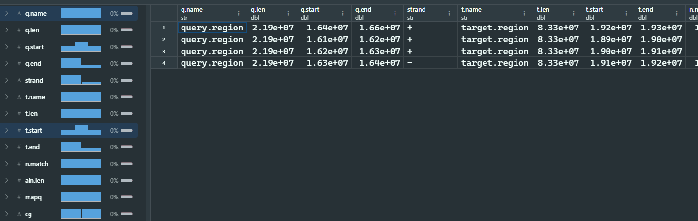
3 读取和过滤PAF文件
3.1 读取
1
2
3
4
5
6
7
8
9
10
11
12
13
14
15
|
paf.file <- system.file("extdata", "test1.paf",package = "SVbyEye")
paf.table <- readPaf(
paf.file = paf.file,
include.paf.tags = TRUE, restrict.paf.tags = "cg"
)
paf.table
|
3.2 过滤
1
2
| ## 基于比对的大小进行筛选
filterPaf(paf.table = paf.table, min.align.len = 100000)
|
3.3 转换
1
2
| ## 强制调换PAF比对结果中的链特征
flipPaf(paf.table = paf.table, force = TRUE)
|
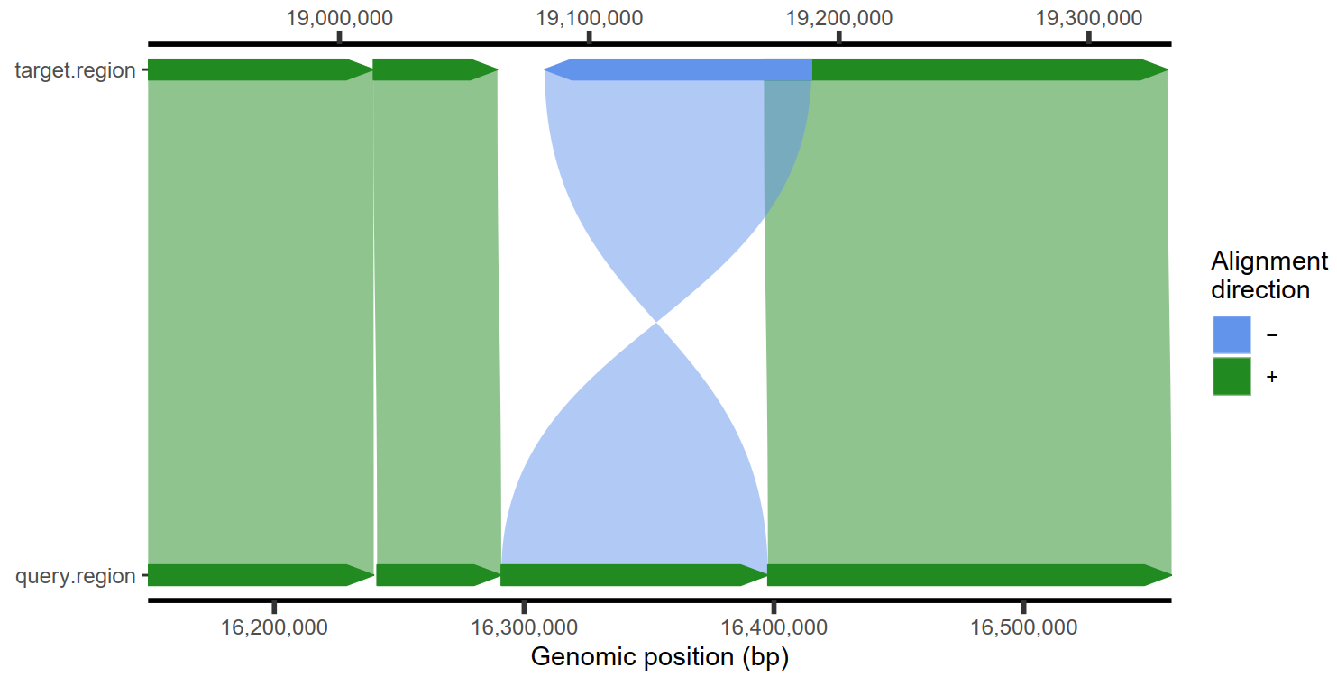
4 sequence-to-sequence比对结果可视化
可视化的主要函数是plotMiro(),可以可视化一个序列比对到参考基因组的结果,也可以可视化两个及以上序列相互比对的结果。这个函数输出的图像是水平的,最上面的是target sequence,下面的是query sequence.
1
2
3
4
5
6
7
8
9
10
11
12
13
14
15
16
17
| library(SVbyEye)
## Get PAF to plot
paf.file <- system.file("extdata", "test1.paf",
package = "SVbyEye"
)
## Read in PAF
paf.table <- readPaf(
paf.file = paf.file,
include.paf.tags = TRUE, restrict.paf.tags = "cg"
)
paf.table
## Make a plot colored by alignment directionality
plotMiro(paf.table = paf.table, color.by = "direction")
|
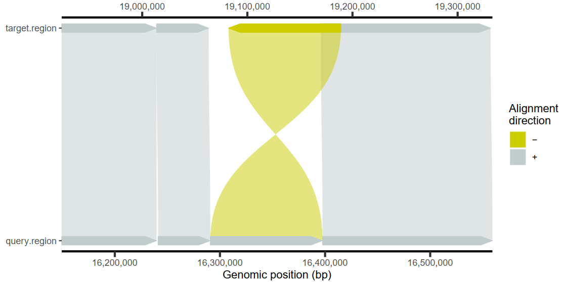
1
2
| # 设置颜色
plotMiro(paf.table = paf.table, color.palette = c("+" = "azure3", "-" = "yellow3"))
|
1
2
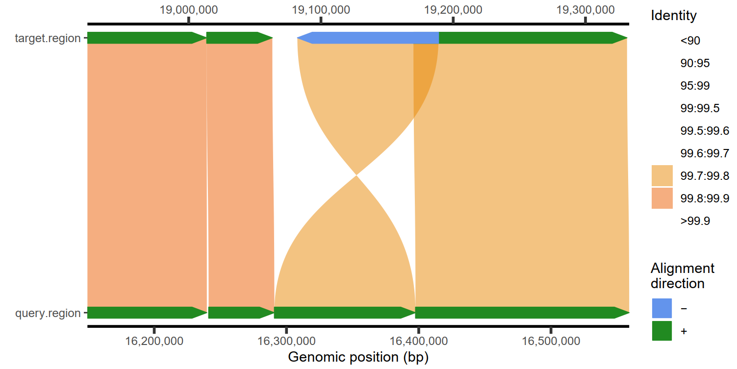
| # 使用相似度上色,而不是方向
plotMiro(paf.table = paf.table, color.by = "identity")
|
1
2
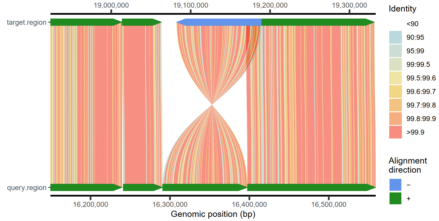
| # 设置划窗的大小
plotMiro(paf.table = paf.table, binsize = 1000)
|
4.1 添加注释信息
1
2
3
4
5
6
7
8
9
| ## Make a plot
plt <- plotMiro(paf.table = paf.table)
## Load target annotation file
target.annot <- system.file("extdata", "test1_target_annot.txt", package = "SVbyEye")
target.annot.df <- read.table(target.annot, header = TRUE, sep = "\t", stringsAsFactors = FALSE)
target.annot.gr <- GenomicRanges::makeGRangesFromDataFrame(target.annot.df)
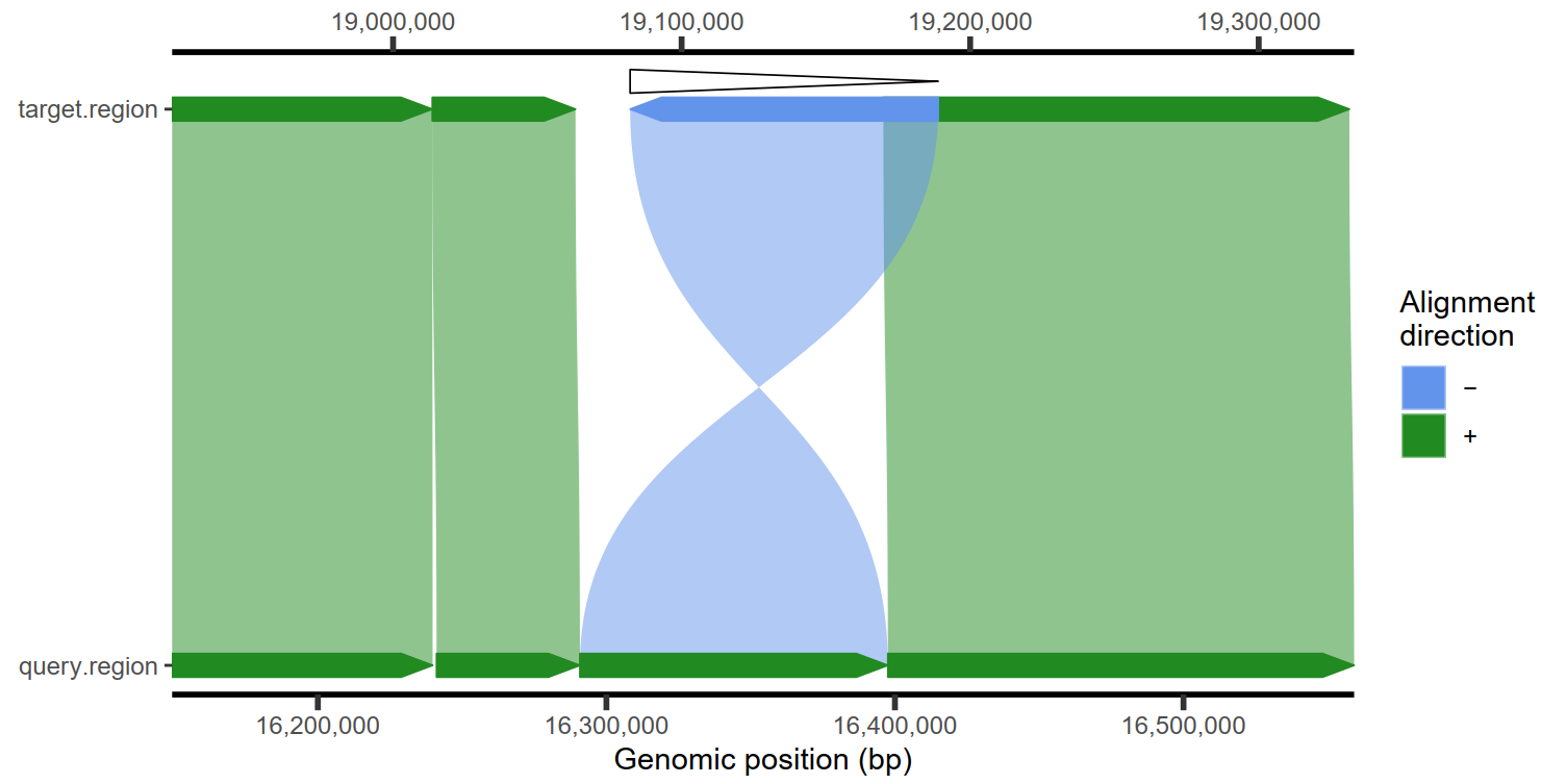
## Add target annotation as arrowhead
addAnnotation(ggplot.obj = plt, annot.gr = target.annot.gr, coordinate.space = "target")
|
1
2
3
4
5
6
7
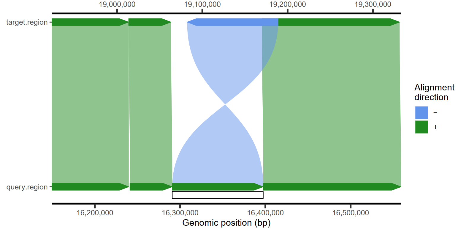
| ## Load query annotation file
query.annot <- system.file("extdata", "test1_query_annot.txt", package = "SVbyEye")
query.annot.df <- read.table(query.annot, header = TRUE, sep = "\t", stringsAsFactors = FALSE)
query.annot.gr <- GenomicRanges::makeGRangesFromDataFrame(query.annot.df)
## Add query annotation as rectangle
addAnnotation(ggplot.obj = plt, annot.gr = query.annot.gr, shape = "rectangle", coordinate.space = "query")
|
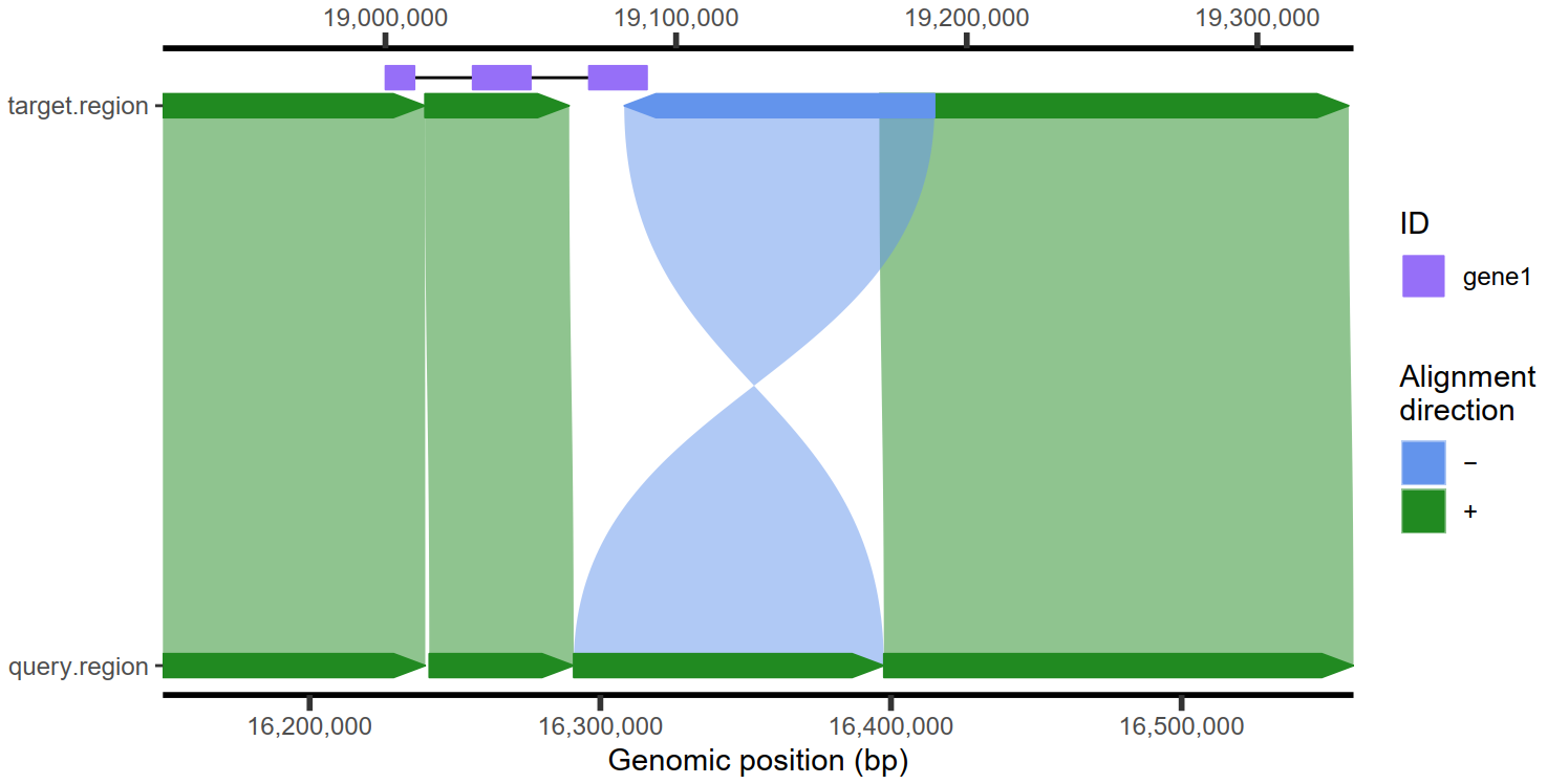
4.2 添加基因注释信息
1
2
3
4
5
6
7
8
9
| ## Create gene-like annotation
test.gr <- GenomicRanges::GRanges(
seqnames = 'target.region',
ranges = IRanges::IRanges(start = c(19000000,19030000,19070000),
end = c(19010000,19050000,19090000)),
ID = 'gene1')
## Add single gene annotation
addAnnotation(ggplot.obj = plt, annot.gr = test.gr, coordinate.space = "target",shape = 'rectangle', annotation.group = 'ID', fill.by = 'ID')
|
4.3 强调某个部分
1
2
3
4
5
6
7
| ## Make a plot
plt1 <- plotMiro(paf.table = paf.table, add.alignment.arrows = FALSE)
## Highlight alignment as a filled polygon
addAlignments(ggplot.obj = plt1, paf.table = paf.table[3,], fill.by = 'strand',
fill.palette = c('+' = 'red'))
addAlignments(ggplot.obj = plt1, paf.table = paf.table[4,], linetype = 'dashed')
|
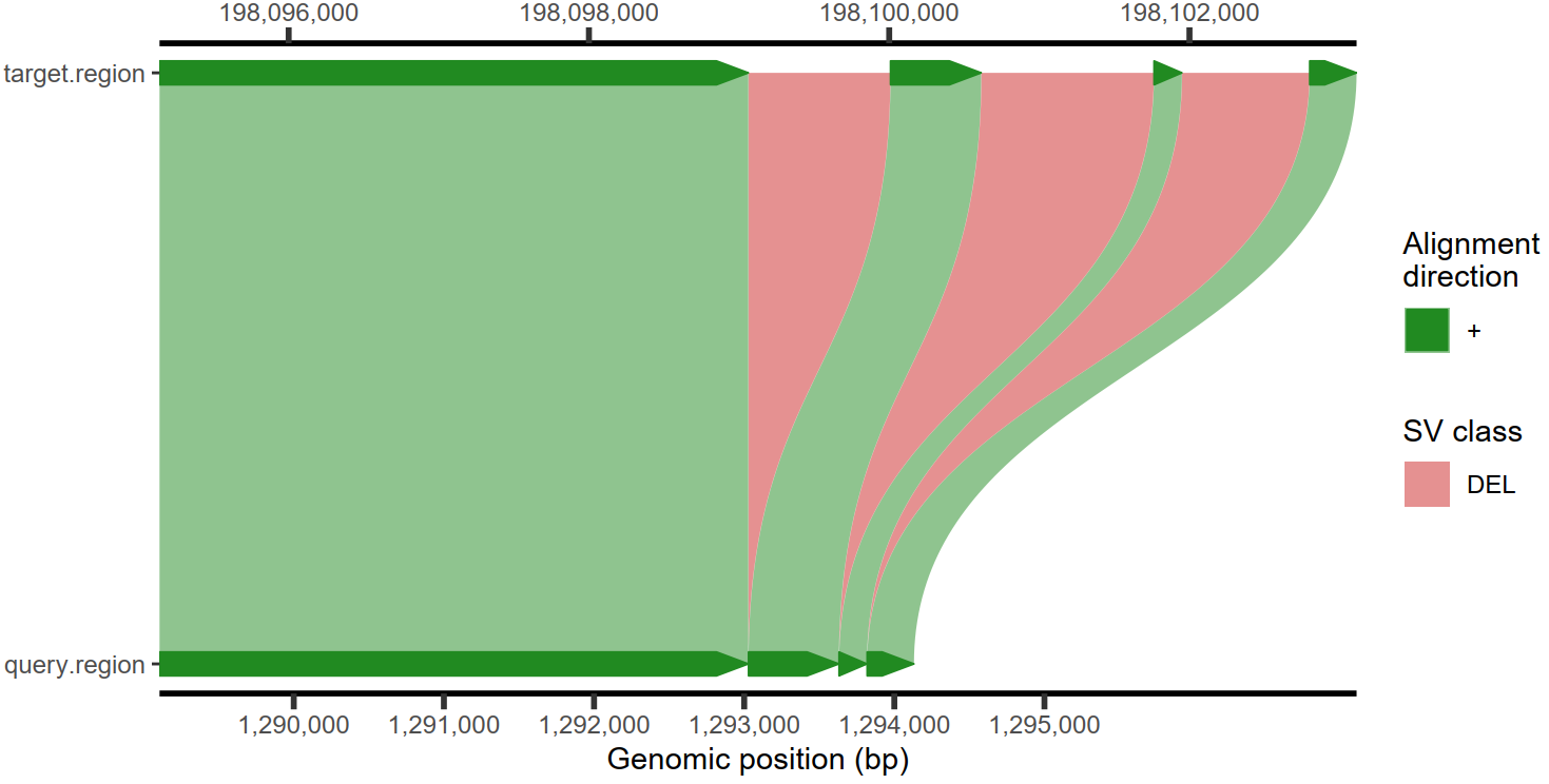
4.4 插入和缺失检测与可视化
1
2
| plotMiro(paf.table = paf.table, min.deletion.size = 50, highlight.sv = "fill") -> p
ggsave(p, file = "D:/OneDrive/桌面/4.pdf", width = 8, height = 4, dpi = 500, bg = "white")
|
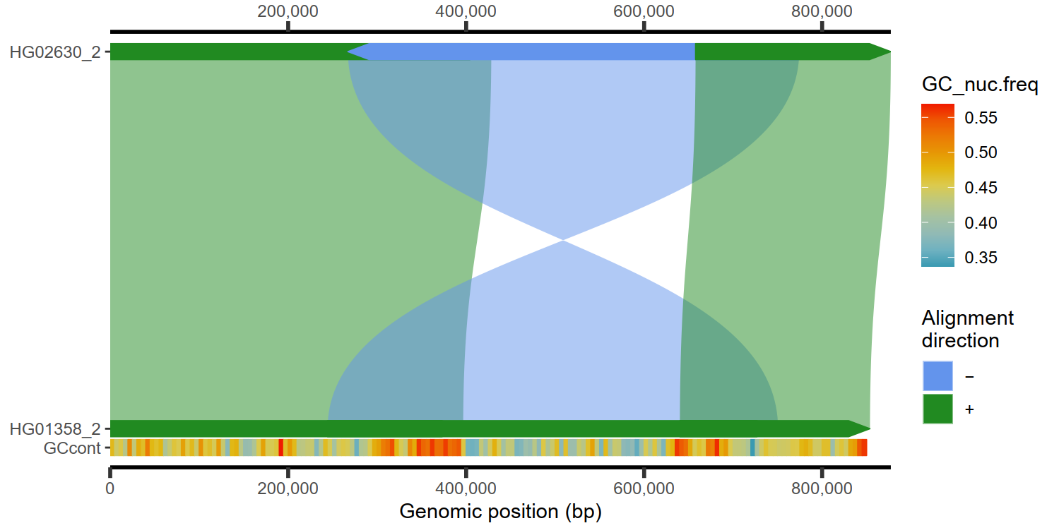
4.5 热图展示GC含量
1
2
3
4
5
6
7
8
9
10
11
12
13
14
15
16
17
18
19
20
21
22
23
24
25
26
|
paf.file <- system.file("extdata", "test_getFASTA.paf",
package = "SVbyEye"
)
paf.table <- readPaf(
paf.file = paf.file,
include.paf.tags = TRUE, restrict.paf.tags = "cg"
)
plt <- plotMiro(paf.table = paf.table, color.by = "direction")
fa.file <- paf.file <- system.file("extdata", "test_getFASTA_query.fasta",
package = "SVbyEye"
)
gc.content <- fasta2nucleotideContent(fasta.file = fa.file,
binsize = 5000, nucleotide.content = 'GC')
addAnnotation(ggplot.obj = plt, annot.gr = gc.content, shape = 'rectangle',
fill.by = 'GC_nuc.freq', coordinate.space = 'query', annotation.label = 'GCcont')
|
4.6 多序列比对结果
1
2
3
4
5
6
7
| ## Get PAF to plot
paf.file <- system.file("extdata", "test_ava.paf", package = "SVbyEye")
## Read in PAF
paf.table <- readPaf(paf.file = paf.file, include.paf.tags = TRUE, restrict.paf.tags = "cg")
plotAVA(paf.table = paf.table, binsize = 20000)
|

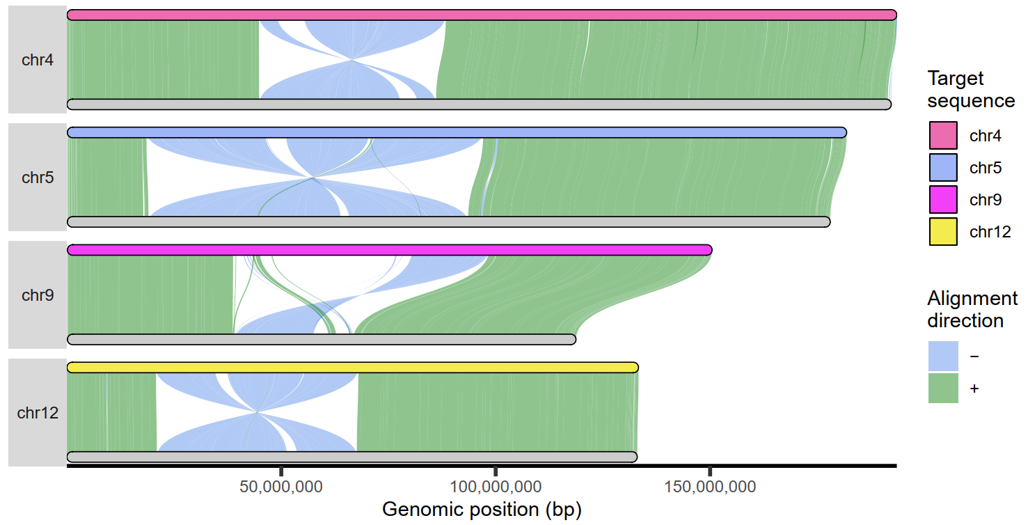
5 全基因组比对可视化
1
2
3
4
5
6
7
8
9
| ## Get PAF to plot ##
paf.file <- system.file("extdata", "PTR_test.paf", package = "SVbyEye")
## Read in PAF
paf.table <- readPaf(paf.file = paf.file)
## Color by alignment directionality
plotGenome(paf.table = paf.table, chromosomes = paste0('chr', c(4, 5, 9, 12)), chromosome.bar.width = grid::unit(2, 'mm'), min.query.aligned.bp = 5000000)
|